LSTM으로 스팸메일 분류하기

이번에는 "딥러닝을 이용한 자연어 처리 입문"에 게재된 스팸메일 분류하기를 통해 자연어처리(NLP)의 과정을 정리해보고자 한다.

본 내용은 10장의 RNN을 이용한 텍스트 분류의 내용이다.

https://wikidocs.net/book/2155

< 자연어 처리 기본 순서 >

1. 데이터의 샘플 수 확인하기 ( 데이터 크기 확인 )
2. 데이터 타입과 결측값 확인
3. 데이터 레이블 분포 확인
4. train데이터와 test데이터 생성
5. 토큰화
6. 단어등장 빈도 확인 ( 빈도수가 적은 단어 제거 )
7. LSTM으로 스팸 메일 분류

 

필요 라이브러리 설치

import numpy as np
import pandas as pd
import matplotlib.pyplot as plt
import urllib.request
from sklearn.model_selection import train_test_split
from tensorflow.keras.preprocessing.text import Tokenizer
from tensorflow.keras.preprocessing.sequence import pad_sequences

데이터의 샘플 수 확인하기 ( 데이터 크기 확인 )

# 데이터 다운로드
urllib.request.urlretrieve("https://raw.githubusercontent.com/ukairia777/tensorflow-nlp-tutorial/main/10.%20RNN%20Text%20Classification/dataset/spam.csv", filename="spam.csv")
data = pd.read_csv('spam.csv', encoding='latin1')
print('총 샘플의 수 :',len(data))

아무 데이터가 없는 컬럼 Unamed: 2, Unamed: 3, Unamed: 4를 지워줍니다.

del data['Unnamed: 2']
del data['Unnamed: 3']
del data['Unnamed: 4']
data['v1'] = data['v1'].replace(['ham','spam'],[0,1])
data[:5]

데이터 타입과 결측값 확인

data.info()

print('결측값 여부 :',data.isnull().values.any())
''' 결측값 여부 : False '''
print('v2열의 유니크한 값 :',data['v2'].nunique())
''' v2열의 유니크한 값 : 5169 '''
data.drop_duplicates(subset=['v2'], inplace=True)
print('총 샘플의 수 :',len(data))
''' 총 샘플의 수 : 5169 '''

데이터 레이블 분포 확인

data['v1'].value_counts().plot(kind='bar')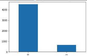

레이블 값 분포

print('정상 메일과 스팸 메일의 개수')
print(data.groupby('v1').size().reset_index(name='count'))
'''
정상 메일과 스팸 메일의 개수
   v1  count
0   0   4516
1   1    653 '''

print(f'정상 메일의 비율 = {round(data["v1"].value_counts()[0]/len(data) * 100,3)}%')
print(f'스팸 메일의 비율 = {round(data["v1"].value_counts()[1]/len(data) * 100,3)}%')
'''
정상 메일의 비율 = 87.367%
스팸 메일의 비율 = 12.633% '''

train데이터와 test데이터 생성

X_data = data['v2']
y_data = data['v1']
print('메일 본문의 개수: {}'.format(len(X_data)))
print('레이블의 개수: {}'.format(len(y_data)))
'''
--------훈련 데이터의 비율-----------
정상 메일 = 87.376%
스팸 메일 = 12.624% '''

# train과 test의 x값과 y값 구분
X_train, X_test, y_train, y_test = train_test_split(X_data, y_data, test_size=0.2, random_state=0, stratify=y_data)


print('--------테스트 데이터의 비율-----------')
print(f'정상 메일 = {round(y_test.value_counts()[0]/len(y_test) * 100,3)}%')
print(f'스팸 메일 = {round(y_test.value_counts()[1]/len(y_test) * 100,3)}%')
'''
--------테스트 데이터의 비율-----------
정상 메일 = 87.331%
스팸 메일 = 12.669% '''

토큰화

tokenizer = Tokenizer()
tokenizer.fit_on_texts(X_train)
X_train_encoded = tokenizer.texts_to_sequences(X_train)

word_to_index = tokenizer.word_index

단어등장 빈도 확인 ( 빈도수가 적은 단어 제거 가능 )

threshold = 2
total_cnt = len(word_to_index) # 단어의 수
rare_cnt = 0 # 등장 빈도수가 threshold보다 작은 단어의 개수를 카운트
total_freq = 0 # 훈련 데이터의 전체 단어 빈도수 총 합
rare_freq = 0 # 등장 빈도수가 threshold보다 작은 단어의 등장 빈도수의 총 합

# 단어와 빈도수의 쌍(pair)을 key와 value로 받는다.
for key, value in tokenizer.word_counts.items():
    total_freq = total_freq + value

    # 단어의 등장 빈도수가 threshold보다 작으면
    if(value < threshold):
        rare_cnt = rare_cnt + 1
        rare_freq = rare_freq + value

print('등장 빈도가 %s번 이하인 희귀 단어의 수: %s'%(threshold - 1, rare_cnt))
print("단어 집합(vocabulary)에서 희귀 단어의 비율:", (rare_cnt / total_cnt)*100)
print("전체 등장 빈도에서 희귀 단어 등장 빈도 비율:", (rare_freq / total_freq)*100)

'''
등장 빈도가 1번 이하인 희귀 단어의 수: 4337
단어 집합(vocabulary)에서 희귀 단어의 비율: 55.45326684567191
전체 등장 빈도에서 희귀 단어 등장 빈도 비율: 6.65745644331875 '''

vocab_size = len(word_to_index) + 1
print('단어 집합의 크기: {}'.format((vocab_size)))
''' 
단어 집합의 크기: 7822 '''

print('메일의 최대 길이 : %d' % max(len(sample) for sample in X_train_encoded))
print('메일의 평균 길이 : %f' % (sum(map(len, X_train_encoded))/len(X_train_encoded)))
plt.hist([len(sample) for sample in X_data], bins=50)
plt.xlabel('length of samples')
plt.ylabel('number of samples')
plt.show()
'''
메일의 최대 길이 : 189
메일의 평균 길이 : 15.754534 '''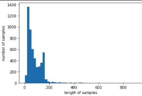

문장 별 단어 길이

#문장 최대 길이가 189임으로, 크기를 189로 동일하게 만들기 위해 빈 공간 패딩
max_len = 189
X_train_padded = pad_sequences(X_train_encoded, maxlen = max_len)
print("훈련 데이터의 크기(shape):", X_train_padded.shape)

LSTM으로 스팸 메일 분류

 

학습

from tensorflow.keras.layers import SimpleRNN, Embedding, Dense
from tensorflow.keras.models import Sequential

embedding_dim = 32
hidden_units = 32

model = Sequential()
model.add(Embedding(vocab_size, embedding_dim))
model.add(SimpleRNN(hidden_units))
model.add(Dense(1, activation='sigmoid'))

model.compile(optimizer='rmsprop', loss='binary_crossentropy', metrics=['acc'])
history = model.fit(X_train_padded, y_train, epochs=4, batch_size=64, validation_split=0.2)

평가

X_test_encoded = tokenizer.texts_to_sequences(X_test)
X_test_padded = pad_sequences(X_test_encoded, maxlen = max_len)
print("\n 테스트 정확도: %.4f" % (model.evaluate(X_test_padded, y_test)[1]))

시각화

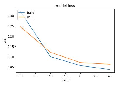
epochs = range(1, len(history.history['acc']) + 1)
plt.plot(epochs, history.history['loss'])
plt.plot(epochs, history.history['val_loss'])
plt.title('model loss')
plt.ylabel('loss')
plt.xlabel('epoch')
plt.legend(['train', 'val'], loc='upper left')
plt.show()